Substitution reactions can be labile or nonlabile
Labile reaction proceed rapidly, with half-lives less than a minute (or so)
Nonlabile (or inert) complexes either do not react or react with half-lives greater than a minute
Lability generally follows the LFSE: large LFSE complexes tend to be nonlabile and small LFSE complexes are labile
A generic substitution reaction for octahedral complex can be written as
[ML6] + X → [ML5X] + L
Thermodynamically, this reaction will be favored if X is a stronger ligand than L; this is an enthalpic effect
The reaction also be favored if ring formation occurs:
[ML6] + X—X → [ML4(X—X)] + 2 L
Ring formation is an entropic effect, so the reaction can be favored even if the X binding site is a weaker ligand than L.
Recall that for consecutive substitution reactions from aqueous media are usually equilibria, with equilibrium constants defined by formation constants, Kf
[M(H2O)6] + X ⇄ [M(H2O)5X] + H2O Kf1 = [M(H2O)5X]/[M(H2O)6][X]
[M(H2O)5X] + X ⇄ [M(H2O)4X2] + H2O Kf2 = [M(H2O)4X2]/[M(H2O)5X][X]
[M(H2O)4X2] + X ⇄ [M(H2O)3X3] + H2O Kf3 = [M(H2O)3X3]/[M(H2O)4X2][X]
etc
The net equilibirum constant is denoted β = Kf1Kf2Kf3···
In most cases the first 5 substitutions are favorable but the 6th position is difficult to occupy.
These are sometimes reported as dissociation constants: Kd = 1/Kf
In square planar complexes an initial substitution is similar to what happens in an Oh complex.
However, the second substitution is often not statistical. Rather, the second substitution is directed by the existing ligands. A strong σ-donor ligand or a strong π-acceptor ligand directs the substitution trans to the directing ligand. This is known as the trans effect
For example, suppose L is a strong σ-donor and X is a weak σ-donor
[ML4] + X → [ML3X] + L
[ML3X] + X → cis-[ML2X2] + L
The effectiveness of trans-directing for σ-donors is: OH– < NH3 < Cl– < Br– < CN– ~ CH3– < I– < SCN– < PR3 ~ H–
For π acceptors, the order is: Br– < I– < NCS– < NO2– < CN– < CO ~ C2H4
Substitution reaction are typically categorized into three categories:
Associative (A) – this is analogous to SN2 reactions in organic chemistry
Dissociative (D) – this is analogous to SN1 reactions in organic chemistry
Interchange (I) – this is analogous to concerted reactions in organic chemistry
In this mechanism the ligand to be added bonds to the metal complex to form an intermediate. The intermediate then breaks apart with the leaving group being one of the products. In terms of reactions:
[ML6] + X ⇄ k1 k–1 [ML6,X]
[ML6,X] → k2 [ML5X] + L
If the first step is the slow step, then the rate law is Rate = d[ML6]/dt = –k1[ML6][X] + k–1[ML6,X]
Since the second step is fast, the [ML6,X] ~ 0
So the net rate law is d[ML6]/dt = –k1[ML6][X]
Running the reaction is a large excess of X (pseudo-first order conditions) gives d[ML6]/dt = –kobs[ML6] where kobs = k1[X]
A plot of kobs vs [X] has a slope of k1 and an intercept of 0
If the second step is the slow step the rate law is: d[ML6]/dt = d[ML6,X]/dt = –k2[ML6,X]
The fast equilibrium can be used to eliminate the intermediate: [ML6,X] = k1[ML6][X]/k–1
Giving: d[ML6]/dt = –k1k2[ML6][X]/k–1 = –kobs[ML6][X]
Running the reaction is a large excess of X (pseudo-first order conditions) gives d[ML6]/dt = –kobs[ML6] where kobs = k1k2/k–1[X]
A plot of kobs vs [X] has a slope of k1k2/k–1 and an intercept of 0
The nature of the initial associated complex can be strongly bonded ([ML6,X] = [ML6X]) or weakly bonded. When the association is weak such that the "complex" is better thought of as an encounter complex, the approximations made above are not valid. This is known as the Eigen-Wilkins mechanism.
Under the conditions of an encounter complex, the substituting the concentration of the intermediate simply using the equilibrium reaction is not valid. Rather, [ML6,X] + [ML6] = [ML6]o
Then, [ML6,X] = k1[ML6][X]/k–1 becomes
[ML6,X] = k1{[ML6]o – [ML6,X]}[X]/k–1
Solving: [ML6,X] = (k1/k–1)[ML6]o[X]/(1 + (k1/k–1)[X])
So that d[ML6]/dt = (k1/k–1)k2[ML6]o[X]/(1 + (k1/k–1)[X])
d[ML6]/dt = kobs[ML6]o
where kobs = k1k2[X]/(k–1 + k1[X])
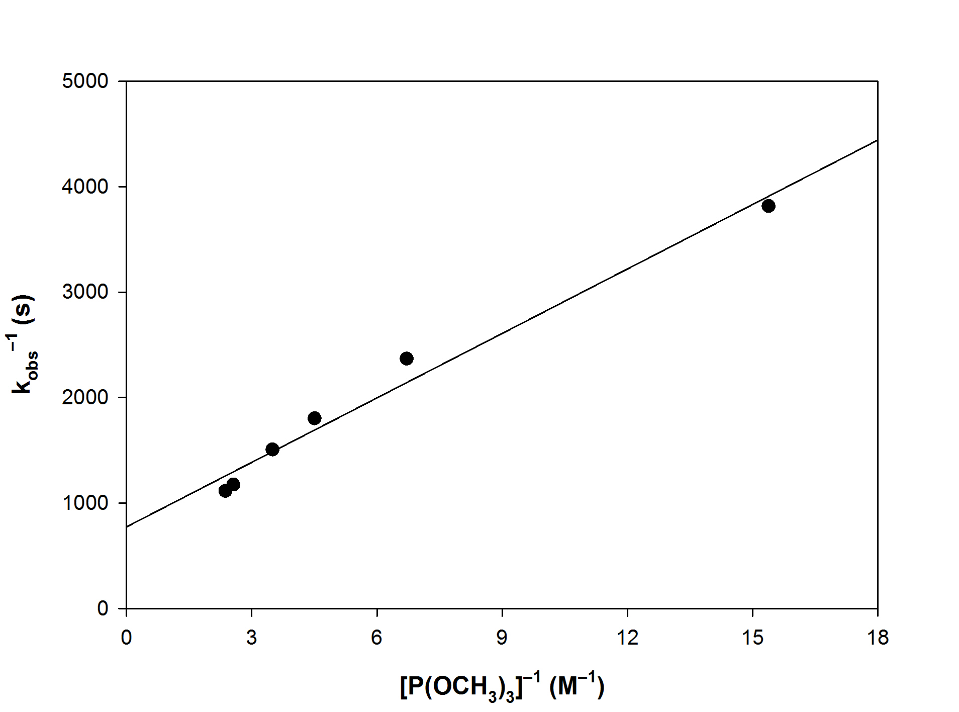
A plot of kobs–1 vs [X]–1 is linear where the slope is k–1/k1k2 and the intercept is 1/k2
Here, the rate determining step is the dissociation of the leaving group from the initial complex giving an coordinately unsaturated intermediate that, in principle, can be detected.
If the dissociation is not an equilibrium, then the mechanism can be written as
[ML6] → k1 [ML5] + L
[ML5] + X → k2 [ML5X]
Under this scenario, the rate law is simple: d[ML6]/dt = –k1[ML6]
This is unusual.
If the initial dissociation is an equilibrium, then
[ML6] ⇄ k1 k–1 [ML5] + L
[ML5] + X → k2 [ML5X]
If the first step is the slow step
The rate law is given by d[ML6]/dt = –k1[ML6] (the intermediate disappears quickly, as above)
If the second step is the slow step
The rate law is given by d[ML6]/dt = –k1[ML5][X]
Under steady state conditions, the concentration of the intermediate is found from d[ML5]/dt = 0 = k1[ML6] – k–1[ML5][L]] – k2[ML5][X]
[ML5] = k1[ML6]/(k–1[L] + k2[X])
So that d[ML6]/dt = –k1k2[ML6][X]/(k1[L] + k2[X])
If the second step is slow, then the intermediate often can be observed experimentally so the second reaction can be monitored directly
The (A) and (I) mechanisms are similar. The difference is based on the lifetime of the intermediate, i.e. k2 (I) >> k2 (A)
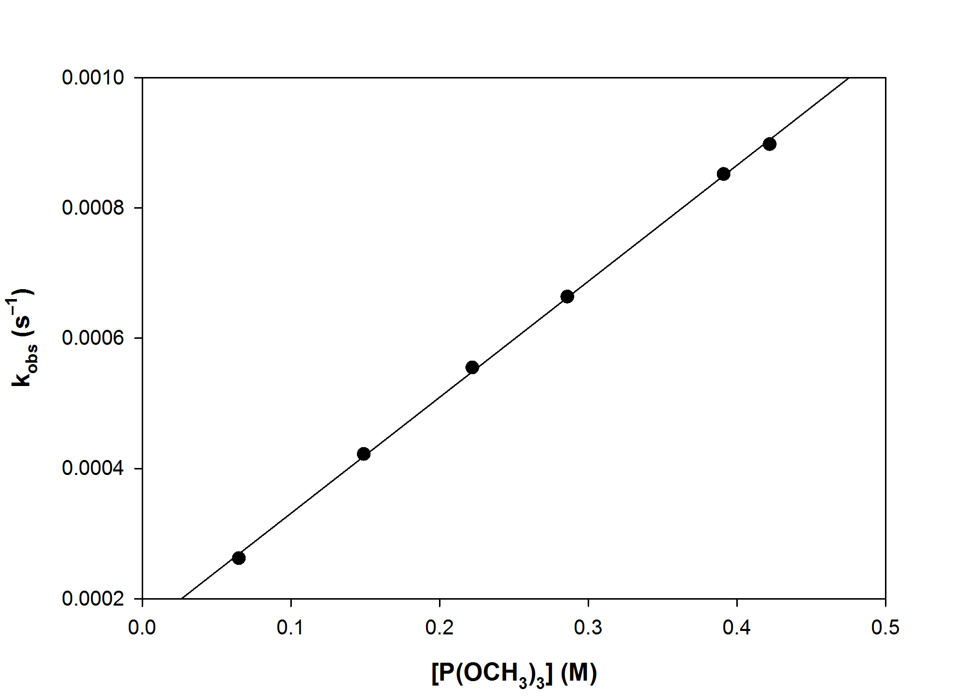
Consider the reaction
[(η5-C9H7Mo(CO)3Br] + P(OCH3)3 → [(η5-C9H7Mo(CO)3(P(OCH3)3)]+ + Br–
The following data was reported (A. J.Hart-Davis, C. White, R. H. Mawby, Inorg. Chim. Acta, 1970, 4, 441)
[P(OCH3)3] (M)
kobs (s–1)
0.065
2.62×10⁻⁴
0.149
4.22×10⁻⁴
0.222
5.55×10⁻⁴
0.286
6.64×10⁻⁴
0.391
8.52×10⁻⁴
0.422
8.98×10⁻⁴
What is the likely mechanism?
Since there is a dependence of the rate constant on the entering ligand, the mechanism is likely to be either A or I
Plotting kobs vs [P(OCH3)3] and kobs–1 vs [P(OCH3)3]–1
The linear plot is the simple A mechanism, not the Eigen-Wilks case. The data does not indicate the slow step.