
Choose the data set corresponding to the last digit of your Student ID Number.
The data given is the solubility in g/L for the indicated salt at each temperature. Use this data to find the ΔH° and ΔS° for the solubilization of the salt by using a van't Hoff plot. Find the slope and intercept graphically, using all of the data. Using the data from the Table of Thermodynamic Quantities, compare the calculated values for ΔH° and ΔS° to those found from your graph. Is the agreement good, bad, or indifferent?
Hints:
Write the reaction. This is critical for solving this problem correctly.
Note units of the solubility. You will need to find the equilibrium constant from the solubility, which we did not do in class. Recall that mass action expressions are expressed in terms of molarity and use the principals described earlier.
For finding the slope and intercept, use the techniques we used earlier for Arrhenius plots of kinetic data.
To find ΔH° and ΔS° from data in the Table of Thermodynamic Quantities, follow the procedures in Homework 24 and Homework 25.
If you are assigned one of the mercury salts, note that Hg22+ is a single ion that contains two atoms. The mercury does not break apart into 2 Hg+ ions.
This is a long homework assignment and integrates ideas from several parts of the course, so will be worth 20 points.
Table of solubilities of various salts in water as a function of temperature.
Set01 234 567 89
T (°C)MgF2 (g/L) CaF2 (g/L)SrF2 (g/L) BaF2 (g/L)PbCl2 (g/L) PbBr2 (g/L)PbI2 (g/L) Hg2Cl2 (g/L) Hg2Br2 (g/L) Hg2I2 (g/L)
50.0157 0.02150.1280.477 4.352.700.314 0.0001342.86×10–6 3.48×10⁻⁸
150.0167 0.02020.1150.459 3.932.170.450 0.0001935.79×10–6 7.57×10⁻⁸
250.0155 0.02270.1240.483 4.823.130.601 0.0003179.81×10–6 1.53×10⁻⁷
350.0145 0.02410.1310.511 5.443.630.812 0.0005341.47×10–5 3.81×10⁻⁷
450.0143 0.02540.1370.503 6.004.260.953 0.0008063.63×10–5 6.58×10⁻⁷
550.0138 0.02640.1330.527 6.434.761.27 0.001395.87×10–5 9.96×10⁻⁷
650.0136 0.02780.1510.542 7.075.471.56 0.001806.65×10–5 1.89×10⁻⁶
750.0130 0.02870.1410.556 7.675.721.94 0.002221.23×10–4 6.54×10⁻⁶
850.0127 0.02950.1530.578 8.167.242.58 0.002221.89×10–4 8.48×10⁻⁶
950.0123 0.03050.1510.576 8.807.773.28 0.004613.89×10–4 1.27×10⁻⁵
MgF2
The reaction is: MgF2(s) → ← Mg2+(aq) + 2 F –(aq)
The molar solubilities of magnesium fluoride are found by dividing the given mass solubilites (g/L) by the molar mass, 62.3 g/mol. Since this is a 1:2 salt, Ksp = [Mg2+]e[F –]e2 = 4s3, where s is the molar solubility.
|
|
|
|
|
|
|
|
|
|
|
|
|
|
|
|
|
|
|
|
|
|
|
|
|
|
|
|
|
|
|
|
|
|
|
|
|
|
|
|
|
|
|
|
|
|
|
|
|
|
|
|
|
|
|
|
|
|
|
|
|
|
|
|
|
|
|
|
|
|
|
|
|
|
|
|
|
|
|
|
|
|
|
|
|
|
|
|
The highlighted cells are plotted, as shown below:
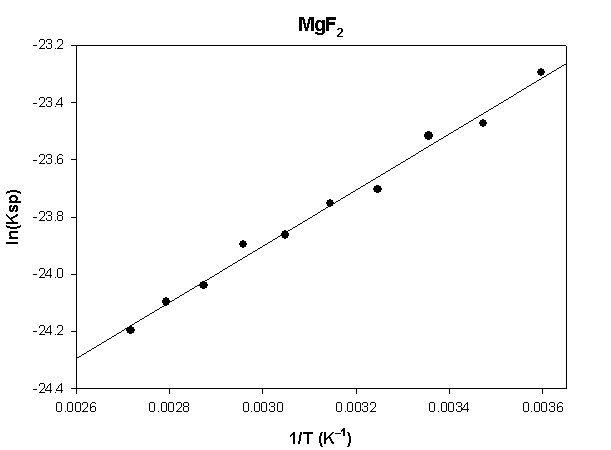
The slope of the plot = 984 and the intercept is –26.9.
ΔH° = –R×slope = –8.314×(984) = 8180 J = –8.2 kJ
ΔS° = R×intercept = 8.314×(–26.9) = –224 J/K
To find the values from the Table of Thermodynamic Quantities :
ΔHf°(Mg2+(aq)) = –466.9 kJ/mol
ΔHf°(F –(aq)) = –332.6 kJ/mol
ΔHf°(MgF2(s)) = –1124 kJ/mol
S°(Mg2+(aq)) = –138.1 J/mol•K
S°(F –(aq)) = –13.8 J/mol•K
S°(MgF2(s)) = 57.24 J/mol•K
ΔH° = [–466.9 + 2(–332.6)] – [–1124] = –8. kJ/mol
ΔS° = [–138.1 + 2(–13.8)] – [57.24] = –222.9 J/mol•K
The agreement is good for the enthalpy change and better than expected for the entropy change.
CaF2
The reaction is: CaF2(s) → ← Ca2+(aq) + 2 F –(aq)
The molar solubilities of calcium fluoride are found by dividing the given mass solubilites (g/L) by the molar mass, 78.1 g/mol. Since this is a 1:2 salt, Ksp = [Ca2+]e[F –]e2 = 4s3, where s is the molar solubility.
|
|
|
|
|
|
|
|
|
|
|
|
|
|
|
|
|
|
|
|
|
|
|
|
|
|
|
|
|
|
|
|
|
|
|
|
|
|
|
|
|
|
|
|
|
|
|
|
|
|
|
|
|
|
|
|
|
|
|
|
|
|
|
|
|
|
|
|
|
|
|
|
|
|
|
|
|
|
|
|
|
|
|
|
|
|
|
|
The highlighted cells are plotted, as shown below:
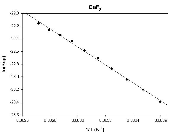
The slope of the plot = –1417 and the intercept is –18.3.
ΔH° = –R×slope = –8.314×(–1417) = 11780 J = 11.8 kJ
ΔS° = R×intercept = 8.314×(–18.3) = –152 J/K
To find the values from the Table of Thermodynamic Quantities :
ΔHf°(Ca2+(aq)) = –542.96 kJ/mol
ΔHf°(F –(aq)) = –332.6 kJ/mol
ΔHf°(CaF2(s)) = –1220 kJ/mol
S°(Ca2+(aq)) = –55.2 J/mol•K
S°(F –(aq)) = –13.8 J/mol•K
S°(CaF2(s)) = 68.87 J/mol•K
ΔH° = [–542.96 + 2(–332.6)] – [–1220.] = 12. kJ/mol
ΔS° = [–55.2 + 2(–13.8)] – [68.87] = –151.7 J/mol•K
The agreement is good for the enthalpy change and better than expected for the entropy change.
SrF2
The reaction is: SrF2(s) → ← Sr2+(aq) + 2 F –(aq)
The molar solubilities of strontium fluoride are found by dividing the given mass solubilites (g/L) by the molar mass, 125.6 g/mol. Since this is a 1:2 salt, Ksp = [Sr2+]e[F –]e2 = 4s3, where s is the molar solubility.
|
|
|
|
|
|
|
|
|
|
|
|
|
|
|
|
|
|
|
|
|
|
|
|
|
|
|
|
|
|
|
|
|
|
|
|
|
|
|
|
|
|
|
|
|
|
|
|
|
|
|
|
|
|
|
|
|
|
|
|
|
|
|
|
|
|
|
|
|
|
|
|
|
|
|
|
|
|
|
|
|
|
|
|
|
|
|
|
The highlighted cells are plotted, as shown below:

The slope of the plot = –656.5 and the intercept is –17.1.
ΔH° = –R×slope = –8.314×(–656.5) = 5458 J = 5.5 kJ
ΔS° = R×intercept = 8.314×(–17.1) = –142 J/K
To find the values from the Table of Thermodynamic Quantities :
ΔHf°(Sr2+(aq)) = –545.8 kJ/mol
ΔHf°(F –(aq)) = –332.6 kJ/mol
ΔHf°(SrF2(s)) = –1216.3 kJ/mol
S°(Sr2+(aq)) = –32.6 J/mol•K
S°(F –(aq)) = –13.8 J/mol•K
S°(SrF2(s)) = 82.1 J/mol•K
ΔH° = [–545.8 + 2(–332.6)] – [–1216.3] = 5.3 kJ/mol
ΔS° = [–32.6 + 2(–13.8)] – [82.1] = –142.3 J/mol•K
The agreement is good for the enthalpy change and better than expected for the entropy change.
BaF2
The reaction is: BaF2(s) → ← Ba2+(aq) + 2 F –(aq)
The molar solubilities of barium fluoride are found by dividing the given mass solubilites (g/L) by the molar mass, 175.3 g/mol. Since this is a 1:2 salt, Ksp = [Ba2+]e[F –]e2 = 4s3, where s is the molar solubility.
|
|
|
|
|
|
|
|
|
|
|
|
|
|
|
|
|
|
|
|
|
|
|
|
|
|
|
|
|
|
|
|
|
|
|
|
|
|
|
|
|
|
|
|
|
|
|
|
|
|
|
|
|
|
|
|
|
|
|
|
|
|
|
|
|
|
|
|
|
|
|
|
|
|
|
|
|
|
|
|
|
|
|
|
|
|
|
|
The highlighted cells are plotted, as shown below:
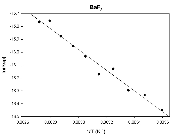
The slope of the plot = –804.2 and the intercept is –13.6.
ΔH° = –R×slope = –8.314×(–804.2) = 6686 J = 6.7 kJ
ΔS° = R×intercept = 8.314×(–13.6) = –113 J/K
To find the values from the Table of Thermodynamic Quantities :
ΔHf°(Ba2+(aq)) = –537.6 kJ/mol
ΔHf°(F –(aq)) = –332.6 kJ/mol
ΔHf°(BaF2(s)) = –1209 kJ/mol
S°(Ba2+(aq)) = 9.6 J/mol•K
S°(F –(aq)) = –13.8 J/mol•K
S°(BaF2(s)) = 96.40 J/mol•K
ΔH° = [–537.6 + 2(–332.6)] – [–1209] = 6. kJ/mol
ΔS° = [9.6 + 2(–13.8)] – [96.40] = –114.4 J/mol•K
The agreement is reasonable for the enthalpy change and better than expected for the entropy change.
PbCl2
The reaction is: PbCl2(s) → ← Pb2+(aq) + 2 Cl –(aq)
The molar solubilities of lead(II) chloride are found by dividing the given mass solubilites (g/L) by the molar mass, 278.2 g/mol. Since this is a 1:2 salt, Ksp = [Pb2+]e[Cl –]e2 = 4s3, where s is the molar solubility.
|
|
|
|
|
|
|
|
|
|
|
|
|
|
|
|
|
|
|
|
|
|
|
|
|
|
|
|
|
|
|
|
|
|
|
|
|
|
|
|
|
|
|
|
|
|
|
|
|
|
|
|
|
|
|
|
|
|
|
|
|
|
|
|
|
|
|
|
|
|
|
|
|
|
|
|
|
|
|
|
|
|
|
|
|
|
|
|
The highlighted cells are plotted, as shown below:
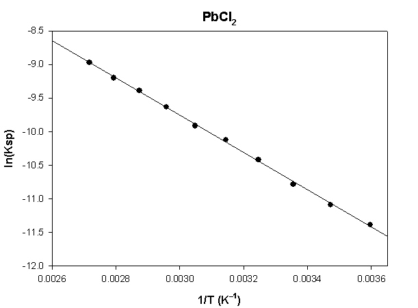
The slope of the plot = –2774 and the intercept is –1.43.
ΔH° = –R×slope = –8.314×(–2774) = 23060 J = –23.1 kJ
ΔS° = R×intercept = 8.314×(–1.43) = –11.9 J/K
To find the values from the Table of Thermodynamic Quantities :
ΔHf°(Pb2+(aq)) = –1.7 kJ/mol
ΔHf°(Cl –(aq)) = –167.2 kJ/mol
ΔHf°(PbCl2(s)) = –359 kJ/mol
S°(Pb2+(aq)) = 10.5 J/mol•K
S°(Cl –(aq)) = 56.5 J/mol•K
S°(PbCl2(s)) = 136 J/mol•K
ΔH° = [–1.7 + 2(–167.2)] – [–359] = 23. kJ
ΔS° = [10.5 + 2(56.5)] – [136] = –13 J/mol•K
The agreement is good for the enthalpy change and better than expected for the entropy change.
PbBr2
The reaction is: PbBr2(s) → ← Pb2+(aq) + 2 Br –(aq)
The molar solubilities of lead(II) bromide are found by dividing the given mass solubilites (g/L) by the molar mass, 367.0 g/mol. Since this is a 1:2 salt, Ksp = [Pb2+]e[Br –]e2 = 4s3, where s is the molar solubility.
|
|
|
|
|
|
|
|
|
|
|
|
|
|
|
|
|
|
|
|
|
|
|
|
|
|
|
|
|
|
|
|
|
|
|
|
|
|
|
|
|
|
|
|
|
|
|
|
|
|
|
|
|
|
|
|
|
|
|
|
|
|
|
|
|
|
|
|
|
|
|
|
|
|
|
|
|
|
|
|
|
|
|
|
|
|
|
|
The highlighted cells are plotted, as shown below:
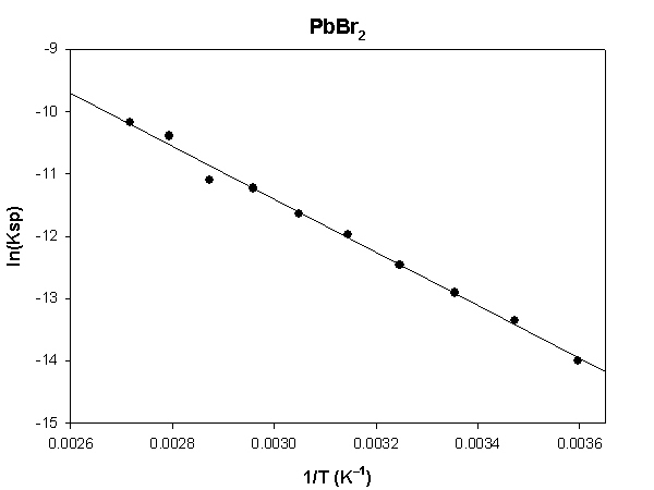
The slope of the plot = –4252 and the intercept is 1.34.
ΔH° = –R×slope = –8.314×(–4252) = 35350 J = 35.4 kJ/mol
ΔS° = R×intercept = 8.314×(1.34) = 11.1 J/K
To find the values from the Table of Thermodynamic Quantities :
ΔHf°(Pb2+(aq)) = –1.7 kJ/mol
ΔHf°(Br –(aq)) = –120.9 kJ/mol
ΔHf°(PbBr2(s)) = –278.7 kJ/mol
S°(Pb2+(aq)) = 10.5 J/mol•K
S°(Br –(aq)) = 80.71 J/mol•K
S°(PbBr2(s)) = 161.5 J/mol•K
ΔH° = [–1.7 + 2(–120.9)] – [–278.7] = 35.2 kJ/mol
ΔS° = [10.5 + 2(80.71)] – [161.5] = 10.4 J/mol•K
The agreement is good for the enthalpy change and better than expected for the entropy change.
PbI2
The reaction is: PbI2(s) → ← Pb2+(aq) + 2 I –(aq)
The molar solubilities of lead(II) iodide are found by dividing the given mass solubilites (g/L) by the molar mass, 461.0 g/mol. Since this is a 1:2 salt, Ksp = [Pb2+]e[I –]e2 = 4s3, where s is the molar solubility.
|
|
|
|
|
|
|
|
|
|
|
|
|
|
|
|
|
|
|
|
|
|
|
|
|
|
|
|
|
|
|
|
|
|
|
|
|
|
|
|
|
|
|
|
|
|
|
|
|
|
|
|
|
|
|
|
|
|
|
|
|
|
|
|
|
|
|
|
|
|
|
|
|
|
|
|
|
|
|
|
|
|
|
|
|
|
|
|
The highlighted cells are plotted, as shown below:

The slope of the plot = –7731 and the intercept is 7.34.
ΔH° = –R×slope = –8.314×(–7731) = 64300 J = 64.3 kJ
ΔS° = R×intercept = 8.314×(7.34) = 61.0 J/K
To find the values from the Table of Thermodynamic Quantities :
ΔHf°(Pb2+(aq)) = –1.7 kJ/mol
ΔHf°(I –(aq)) = –55.19 kJ/mol
ΔHf°(PbI2(s)) = –175.5 kJ/mol
S°(Pb2+(aq)) = 10.5 J/mol•K
S°(I –(aq)) = 111.3 J/mol•K
S°(PbI2(s)) = 174.8 J/mol•K
ΔH° = [–1.7 + 2(–55.19)] – [–175.5] = 63.4 kJ/mol
ΔS° = [10.5 + 2(111.3)] – [174.8] = 58.3 J/mol•K
The agreement is good for the enthalpy change and better than expected for the entropy change.
Hg2Cl2
The reaction is: Hg2Cl2(s) → ← Hg22+(aq) + 2 Cl –(aq)
The molar solubilities of mercury(I) chloride are found by dividing the given mass solubilites (g/L) by the molar mass, 472.2 g/mol. Since this is a 1:2 salt, Ksp = [Hg22+]e[Cl –]e2 = 4s3, where s is the molar solubility.
|
|
|
|
|
|
|
|
|
|
|
|
|
|
|
|
|
|
|
|
|
|
|
|
|
|
|
|
|
|
|
|
|
|
|
|
|
|
|
|
|
|
|
|
|
|
|
|
|
|
|
|
|
|
|
|
|
|
|
|
|
|
|
|
|
|
|
|
|
|
|
|
|
|
|
|
|
|
|
|
|
|
|
|
|
|
|
|
The highlighted cells are plotted, as shown below:
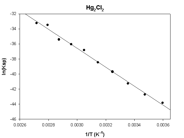
The slope of the plot = –12960 and the intercept is 1.22.
ΔH° = –R×slope = –8.314×(–12960) = 107700 J = 107.7 kJ
ΔS° = R×intercept = 8.314×(1.22) = 10.1 J/K
To find the values from the Table of Thermodynamic Quantities :
ΔHf°(Hg22+(aq)) = 172.4 kJ/mol
ΔHf°(Cl –(aq)) = –167.2 kJ/mol
ΔHf°(Hg2Cl2(s)) = –265.4 kJ/mol
S°(Hg22+(aq)) = 84.5 J/mol•K
S°(Cl –(aq)) = 56.5 J/mol•K
S°(Hg2Cl2(s)) = 191.6 J/mol•K
ΔH° = [172.4 + 2(–167.2)] – [–265.4] = 103.4 kJ/mol
ΔS° = [84.5 + 2(56.5)] – [191.6] = 5.9 J/mol•K
The agreement is modest for both the enthalpy change and the entropy change.
Hg2Br2
The reaction is: Hg2Br2(s) → ← Hg22+(aq) + 2 Br –(aq)
The molar solubilities of mercury(I) bromide are found by dividing the given mass solubilites (g/L) by the molar mass, 561.0 g/mol. Since this is a 1:2 salt, Ksp = [Hg22+]e[Br –]e2 = 4s3, where s is the molar solubility.
|
|
|
|
|
|
|
|
|
|
|
|
|
|
|
|
|
|
|
|
|
|
|
|
|
|
|
|
|
|
|
|
|
|
|
|
|
|
|
|
|
|
|
|
|
|
|
|
|
|
|
|
|
|
|
|
|
|
|
|
|
|
|
|
|
|
|
|
|
|
|
|
|
|
|
|
|
|
|
|
|
|
|
|
|
|
|
|
The highlighted cells are plotted, as shown below:
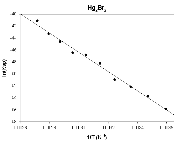
The slope of the plot = –16095 and the intercept is 1.89.
ΔH° = –R×slope = –8.314×(–16095) = 133800 J = 133.8 kJ
ΔS° = R×intercept = 8.314×(1.89) = 15.7 J/K
To find the values from the Table of Thermodynamic Quantities :
ΔHf°(Hg22+(aq)) = 172.4 kJ/mol
ΔHf°(Br –(aq)) = –120.9 kJ/mol
ΔHf°(Hg2Br2(s)) = –206.9 kJ/mol
S°(Hg22+(aq)) = 84.5 J/mol•K
S°(Br –(aq)) = 80.71 J/mol•K
S°(Hg2Br2(s)) = 218.0 J/mol•K
ΔH° = [172.4 + 2(–120.9)] – [–206.9] = 137.5 kJ/mol
ΔS° = [84.5 + 2(80.71)] – [218.0] = 27.9 J/mol•K
The agreement is moderate for the enthalpy change and poor for the entropy change.
Hg2I2
The reaction is: Hg2I2(s) → ← Hg22+(aq) + 2 I –(aq)
The molar solubilities of mercury(I) iodide are found by dividing the given mass solubilites (g/L) by the molar mass, 655.0 g/mol. Since this is a 1:2 salt, Ksp = [Hg22+]e[I –]e2 = 4s3, where s is the molar solubility.
|
|
|
|
|
|
|
|
|
|
|
|
|
|
|
|
|
|
|
|
|
|
|
|
|
|
|
|
|
|
|
|
|
|
|
|
|
|
|
|
|
|
|
|
|
|
|
|
|
|
|
|
|
|
|
|
|
|
|
|
|
|
|
|
|
|
|
|
|
|
|
|
|
|
|
|
|
|
|
|
|
|
|
|
|
|
|
|
The highlighted cells are plotted, as shown below:
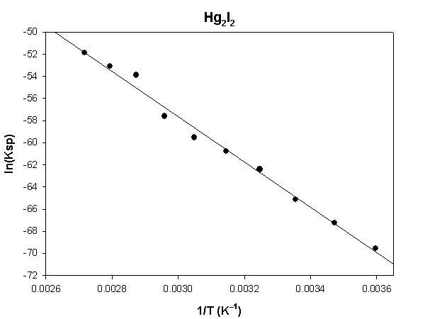
The slope of the plot = –20530 and the intercept is 3.96.
ΔH° = –R×slope = –8.314×(–20530) = 170700 J = 170.7 kJ
ΔS° = R×intercept = 8.314×(3.96) = 32.9 J/K
To find the values from the Table of Thermodynamic Quantities :
ΔHf°(Hg22+(aq)) = 172.4 kJ/mol
ΔHf°(I –(aq)) = –55.19 kJ/mol
ΔHf°(Hg2I2(s)) = –121.3 kJ/mol
S°(Hg22+(aq)) = 84.5 J/mol•K
S°(I –(aq)) = 111.3 J/mol•K
S°(Hg2I2(s)) = 233.5 J/mol•K
ΔH° = [172.4 + 2(–55.19)] – [–121.3] = 183.3 kJ
ΔS° = [84.5 + 2(111.3)] – [233.5] = 73.6 J/mol•K
The agreement is modest for the enthalpy change and poor for the entropy change.